【機械学習】AutoGluonの使い方・クイックスタートの解説(物体検出)

AutoGluonの「物体検出」のクイックスタートについて紹介・解説します。YOLOv3モデルを使って画像からバイクを検出するという内容です。

Object Detection - Quick Start — AutoGluon Documentation 0.2.0 documentation

表形式データや画像認識については別記事で紹介しています。

predora005.hatenablog.com

https://predora005.hatenablog.com/entry/2021/06/20/190000predora005.hatenablog.com

[1] データセットのダウンロード

データセットは、 VOCデータセットの中から、学習用に120枚、検証用に50枚、テスト用に50枚が抽出されたものになっています。

$ curl -OL 'https://autogluon.s3.amazonaws.com/datasets/tiny_motorbike.zip'
$ unzip tiny_motorbike.zip

[2] 学習の実行

データセットを読み込んだのち、学習を実行します。

import autogluon.core as ag
from autogluon.vision import ObjectDetector

url = './tiny_motorbike/'
dataset_train = ObjectDetector.Dataset.from_voc(url, splits='trainval')

num_traialsで学習回数を2回に指定しています。クイックスタートの説明によれば、time_limitでコントールするのが望ましいようです。

time_limit = 60*30  # at most 0.5 hour
detector = ObjectDetector()
hyperparameters = {'epochs': 5, 'batch_size': 8}
hyperparamter_tune_kwargs={'num_trials': 2}
detector.fit(dataset_train, time_limit=time_limit, 
hyperparameters=hyperparameters, 
hyperparamter_tune_kwargs=hyperparamter_tune_kwargs)

終了するまでに、r5.largeインスタンスでは10分、m5.xlargeインスタンスでは 5分ほどかかりました。

[3] 評価・予測の実行

evaluateでテストデータを用いた評価を行います。

dataset_test = ObjectDetector.Dataset.from_voc(url, splits='test')

test_map = detector.evaluate(dataset_test)
print(test_map)
# (['motorbike', 'chair', 'bus', 'car', 'dog', 
#   'bicycle', 'cow', 'person', 'boat', 'pottedplant', 'mAP'], 
#  [0.5806065427876039, nan, 0.47272727272727283, 0.007751937984496126, 
#   0.0, nan, nan, nan, nan, nan, 0.26527143837484324])

mAP (Mean Average Precision)を表示すると、約26%でした。

print("mAP on test dataset: {}".format(test_map[1][-1]))
# mAP on test dataset: 0.26527143837484324

以下では、テストデータから1枚画像を取り出し、予測を実行しています。

image_path = dataset_test.iloc[0]['image']
result = detector.predict(image_path)
print(result)
#    predict_class  predict_score  \
# 0         person       0.972545   
# 1      motorbike       0.656974   
# 2        bicycle       0.413718   
# ..           ...            ...   
# 85        person       0.035410   
# 86        person       0.034698   
# 87       bicycle       0.034663   
# 
#                                          predict_rois  
# 0   {'xmin': 0.3991624116897583, 'ymin': 0.2802912...  
# 1   {'xmin': 0.3347971439361572, 'ymin': 0.4365810...  
# 2   {'xmin': 0.3935226500034332, 'ymin': 0.4864529...  
# ..                                                ...  
# 85  {'xmin': 0.38480135798454285, 'ymin': 0.438172...  
# 86  {'xmin': 0.8661710619926453, 'ymin': 0.4210591...  
# 87  {'xmin': 0.46432197093963623, 'ymin': 0.484336...  
# 
# [88 rows x 3 columns]

検出したオブジェクトのクラス(predict_class)、スコア(predict_score)、バウンディングボックスの位置(predict_rois)が返されます。スコアの良いもののみ可視化すると以下の通りです(ソースコードは補足3に記載しています)。

また、複数枚の画像をまとめて予測することも可能です。

bulk_result = detector.predict(dataset_test)
print(bulk_result)
#      predict_class  predict_score  \
# 0           person       0.972545   
# 1        motorbike       0.656974   
# 2          bicycle       0.413718   
# ...            ...            ...   
# 4594        person       0.034718   
# 4595        person       0.034599   
# 4596        person       0.034501   
# 
#                                            predict_rois  \
# 0     {'xmin': 0.3991624116897583, 'ymin': 0.2802912...   
# 1     {'xmin': 0.3347971439361572, 'ymin': 0.4365810...   
# 2     {'xmin': 0.3935226500034332, 'ymin': 0.4864529...   
# ...                                                 ...   
# 4594  {'xmin': 0.37993040680885315, 'ymin': 0.462566...   
# 4595  {'xmin': 0.9430548548698425, 'ymin': 0.1451357...   
# 4596  {'xmin': 0.4937310814857483, 'ymin': 0.2520754...   
# 
#                                                   image  
# 0     /home/jupyter/tiny_motorbike/JPEGImages/000038...  
# 1     /home/jupyter/tiny_motorbike/JPEGImages/000038...  
# 2     /home/jupyter/tiny_motorbike/JPEGImages/000038...  
# ...                                                 ...  
# 4594  /home/jupyter/tiny_motorbike/JPEGImages/002488...  
# 4595  /home/jupyter/tiny_motorbike/JPEGImages/002488...  
# 4596  /home/jupyter/tiny_motorbike/JPEGImages/002488...  
# 
# [4597 rows x 4 columns]

[4] 分類器のセーブ・ロード

分類器のセーブ・ロードも可能です。savefileで指定したファイル名の通りに保存されます。

savefile = 'detector.ag'
detector.save(savefile)
new_detector = ObjectDetector.load(savefile)

終わりに

学習時間は比較的短めでしたが、それなりの精度は出ているようです。何よりもソースコード数行で物体検出が行えるというのが驚きでした。手軽に物体検出できるのはありがたいです。

出典

• アイキャッチはGerd AltmannによるPixabayからの画像

補足

[補足1] ImportError: libGL.so.1

AutoGluon使用時に以下のエラーが発生することがある。根本はOpenCVがインポートできないことが原因。

ImportError: libGL.so.1: cannot open shared object file: No such file or directory

環境によって解決策が異なるようですが、Amazon Linux2では以下のコマンドで解決しました。

$ sudo yum install -y mesa-libGL.x86_64

[補足2] AutoGluonでデータセットの取得と解凍まで行う

データセットの取得と解凍をプログラムで行うことも可能です。

import autogluon.core as ag
from autogluon.vision import ObjectDetection as task
import os

root = './'
filename_zip = ag.download('https://autogluon.s3.amazonaws.com/datasets/tiny_motorbike.zip',
                        path=root)
filename = ag.unzip(filename_zip, root=root)

data_root = os.path.join(root, filename)
dataset_train = task.Dataset(data_root, classes=('motorbike',))

[補足3] 画像にバインディングボックスとスコアを表示

データセットから画像のパスを取り出し予測させます。次に、予測結果から良いスコアのもののみを取り出しています。ここでは0.7以上を対象としています。

image0_path = dataset_test.iloc[0]['image']
result = detector.predict(image0_path).query('predict_score >= 0.7')

可視化する際に画像をndarrayで渡す必要があります。Pillowで画像を読み込みnp.arrayでndarrayに変換します。

import numpy as np
from PIL import Image

im0 = Image.open(image0_path)
width, height = im0.size
image0 = np.array(im0)

バウンディングボックスは、Nx4のndarrayで渡します。ディクショナリから取り出した座標を画面座標に変換します。

bboxes=[]
for rois in result['predict_rois']:
    x1, y1 = int(rois['xmin']* width), int(rois['ymin']* height)
    x2, y2 = int(rois['xmax']* width), int(rois['ymax']* height)
    bboxes.append([x1, y1, x2, y2])
    
bboxes = np.array(bboxes)

準備したパラメータを渡せば以下のような画像が作れます。

from gluoncv.utils import viz

scores = result['predict_score'].values
labels , class_names = result['predict_class'].factorize()

ax = viz.plot_bbox(image0, bboxes=bboxes, scores=scores, 
                   labels = labels, class_names=class_names)
plt.show()

08. Finetune a pretrained detection model — gluoncv 0.11.0 documentation

【機械学習】AutoGluonの使い方・クイックスタートの解説(画像認識)

AutoGluonの「画像認識」のクイックスタートについて紹介・解説します。

各画像に描かれた衣類のカテゴリーを分類するという内容です。カテゴリはBabyPants, BabyShirt, womencasualshoes, womenchiffontopの4種類です。

Image Prediction - Quick Start — AutoGluon Documentation 0.2.0 documentation

表形式データについては別記事で紹介しています。

predora005.hatenablog.com

[1] データセットのダウンロード

$ curl -OL 'https://autogluon.s3.amazonaws.com/datasets/shopee-iet.zip'
$ unzip shopee-iet.zip

[2] 学習データの確認

学習用データは800枚の画像です。

import autogluon.core as ag
from autogluon.vision import ImagePredictor

train_dataset, _, test_dataset = ImagePredictor.Dataset.from_folders('./data')
print(train_dataset)
#   image  label
# 0    /home/jupyter/data/train/BabyPants/BabyPants_1...      0
# 1    /home/jupyter/data/train/BabyPants/BabyPants_1...      0
# 2    /home/jupyter/data/train/BabyPants/BabyPants_1...      0
# 3    /home/jupyter/data/train/BabyPants/BabyPants_1...      0
# 4    /home/jupyter/data/train/BabyPants/BabyPants_1...      0
# ..                                                 ...    ...
# 795  /home/jupyter/data/train/womenchiffontop/women...      3
# 796  /home/jupyter/data/train/womenchiffontop/women...      3
# 797  /home/jupyter/data/train/womenchiffontop/women...      3
# 798  /home/jupyter/data/train/womenchiffontop/women...      3
# 799  /home/jupyter/data/train/womenchiffontop/women...      3
# 
# [800 rows x 2 columns]

[3] 学習の実行

学習を実行すると、ハイパーパラメータと最適なモデルの選定が自動でおこなれます。 ソース中のコメントにもある通り、学習用データのうち1割が検証用データとして使われます。また、ここでは学習回数(epochs)を2回に制限していますが、制限しない方が良いです。

predictor = ImagePredictor()
# since the original dataset does not provide validation split, the `fit` function splits it randomly with 90/10 ratio
predictor.fit(train_dataset, hyperparameters={'epochs': 2})  # you can trust the default config, we reduce the # epoch to save some build time

学習と検証の予測精度は以下のコードで確認できます。

fit_result = predictor.fit_summary()
print('Top-1 train acc: %.3f, val acc: %.3f' %(fit_result['train_acc'], fit_result['valid_acc']))
# Top-1 train acc: 0.623, val acc: 0.806

[4] 評価の実行

テストデータで評価を行います。

test_acc, _ = predictor.evaluate(test_dataset)
print('Top-1 test acc: %.3f' % test_acc)
# Top-1 test acc: 0.713

[5] 新たな画像のカテゴリを予測

以下は1枚の画像を入力し、どのカテゴリかを確認しています。

image_path = test_dataset.iloc[0]['image']
result = predictor.predict(image_path)
print(result)
# 0    0
# Name: label, dtype: int64

predict_probaで、各カテゴリの予測結果を確認できます。

proba = predictor.predict_proba(image_path)
print(proba)
#           0         1         2         3
# 0  0.498938  0.486701  0.012103  0.002259

複数の画像を入力とし、予測を行うことも可能です。

bulk_result = predictor.predict(test_dataset)
print(bulk_result)
# 0     0
# 1     0
# 2     2
# 3     2
# 4     1
#      ..
# 75    3
# 76    3
# 77    3
# 78    3
# 79    2
# Name: label, Length: 80, dtype: int64

[6] 分類器のセーブ・ロード

以下のように分類器のセーブ・ロードが可能です。

filename = 'predictor.ag'
predictor.save(filename)
predictor_loaded = ImagePredictor.load(filename)
# use predictor_loaded as usual
result = predictor_loaded.predict(image_path)
print(result)
# 0    0
# Name: label, dtype: int64

終わりに

精度がどの程度なのかは分かりませんが、ソースコードはかなり簡単に書くことが出来ました。

出典

• アイキャッチはGerd AltmannによるPixabayからの画像

【機械学習】AutoGluonの使い方・クイックスタートの解説(表形式データ)

「AutoGluon」の使い方を、公式のクイックスタートを解説する形で紹介します。

AutoGluonは、AutoML(Auto Machine Learning)を実現するライブラリです。特徴量の設計など機械学習で大変な部分を自動化してくれます。

AutoGluonは数あるAutoMLライブラリの一種で、テキスト、画像、表データに対応しています。

本記事では、AutoGluonのインストール方法、表形式データのクイックスタートを紹介します。

[1] インストール方法

以下は、LinuxかつGPU無しのインストール手順です。GPU有りや別OSの手順も公式に載っています。

python3 -m pip install -U pip --user
python3 -m pip install -U setuptools wheel --user
python3 -m pip install -U "mxnet<2.0.0" --user
python3 -m pip install autogluon --user

AutoGluon: AutoML for Text, Image, and Tabular Data — AutoGluon Documentation 0.2.0 documentation

[2] クイックスタート

公式では下記4種類のクイックスタートが載っています。

1. 表形式データ
2. 画像分類
3. 物体検出
4. テキスト分類

本記事では、表形式データの内容を紹介します。

[2-1] 概要

ある人の収入が5万ドルを超えるかどうかを予測する分類モデルを作成するという内容です。

Predicting Columns in a Table - Quick Start — AutoGluon Documentation 0.2.0 documentation

[2-2] 学習データの確認

from autogluon.tabular import TabularDataset, TabularPredictor

train_data = TabularDataset('https://autogluon.s3.amazonaws.com/datasets/Inc/train.csv')
subsample_size = 500  # subsample subset of data for faster demo, try setting this to much larger values
train_data = train_data.sample(n=subsample_size, random_state=0)
train_data.head()

500人中、年収5万ドル以下の人が365人、残りの135人が5万ドル以上になります。

label = 'class'
print("Summary of class variable: \n", train_data[label].describe())
# Summary of class variable: 
#  count        500
# unique         2
# top        <=50K
# freq         365
# Name: class, dtype: object

[2-3] 学習の実行

TabularPredictor.fit()で学習を実行します。

save_path = 'agModels-predictClass'  # specifies folder to store trained models
predictor = TabularPredictor(label=label, path=save_path).fit(train_data)
# Summary of class variable: 
#  count        500
# unique         2
# top        <=50K
# freq         365
# Name: class, dtype: object

[2-4] 予測と評価

predictでテストデータを用いた予測を行い、evaluate_predictionsで評価を行います。

test_data = TabularDataset('https://autogluon.s3.amazonaws.com/datasets/Inc/test.csv')
y_test = test_data[label]  # values to predict
test_data_nolab = test_data.drop(columns=[label])  # delete label column to prove we're not cheating
test_data_nolab.head()

predictor = TabularPredictor.load(save_path)  # unnecessary, just demonstrates how to load previously-trained predictor from file
y_pred = predictor.predict(test_data_nolab)
print("Predictions:  \n", y_pred)
# Predictions:  
#  0        <=50K
# 1        <=50K
# 2         >50K
# 3        <=50K
# 4        <=50K
#          ...  
# 9764     <=50K
# 9765     <=50K
# 9766     <=50K
# 9767     <=50K
# 9768     <=50K
# Name: class, Length: 9769, dtype: object

perf = predictor.evaluate_predictions(y_true=y_test, y_pred=y_pred, auxiliary_metrics=True)
# Evaluation: accuracy on test data: 0.8397993653393387
# Evaluations on test data:
# {
#     "accuracy": 0.8397993653393387,
#     "balanced_accuracy": 0.7437076677780596,
#     "mcc": 0.5295565206264157,
#     "f1": 0.6242496998799519,
#     "precision": 0.7038440714672441,
#     "recall": 0.5608283002588438
# }

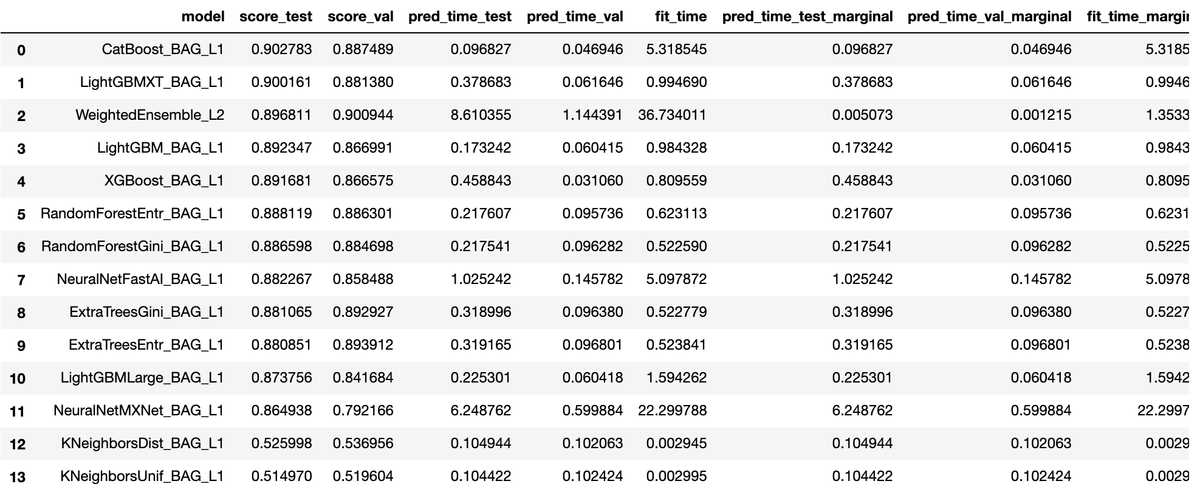
また、leaderboardで訓練を行った各モデルの性能を確認することができます。

predictor.leaderboard(test_data, silent=True)

[2-5] 学習(fit)の中で行われていること

クイックスタートの説明を要約すると次の通りです。

• 二値分類問題であることは自動で認識する。
• どの特徴量が連続値か離散値を自動的に判別する。
• 欠損データや特徴量の再スケーリングなども自動的に処理する。
• 検証用データを使って、複数のモデルを訓練する。
• ハイパーパラメータの選定も自動で行われる。
• 検証用データを指定しない場合は、学習用データからランダムに検証用データを抽出する。

[2-6] 予測精度の最大化

fit()のパラメータを変えることで予測精度の向上を図ることが可能です。

time_limit = 60  # for quick demonstration only, you should set this to longest time you are willing to wait (in seconds)
metric = 'roc_auc'  # specify your evaluation metric here
predictor = TabularPredictor(label, eval_metric=metric).fit(train_data, time_limit=time_limit, presets='best_quality')
predictor.leaderboard(test_data, silent=True)

上記例では、次のことを行っています。

• time_limitで学習時間を60秒まで可能にする。
• metricは評価指標が事前に分かっている場合に指定する。指定できるのはroc_auc, log_loss, mean_absolute_errorなど。
• presetsで精度や速度などの優先順位を指定する。best_qualityは精度優先、デフォルトは'medium_quality_faster_train。

[2-7] 回帰の例

ラベルを年齢('age')にすることで、回帰を行うことも可能です。

age_column = 'age'
print("Summary of age variable: \n", train_data[age_column].describe())
# Summary of age variable: 
#  count    500.00000
# mean      39.65200
# std       13.52393
# min       17.00000
# 25%       29.00000
# 50%       38.00000
# 75%       49.00000
# max       85.00000
# Name: age, dtype: float64

predictor_age = TabularPredictor(label=age_column, path="agModels-predictAge").fit(train_data, time_limit=60)
performance = predictor_age.evaluate(test_data)

predictor_age.leaderboard(test_data, silent=True)

終わりに

あまり細かいことを意識することなく使用することが出来ました。面倒な前処理を自動でやってくれるのは大きいメリットです。

機械学習の精度を向上させるためには、特徴量の作成や選択、モデルのチューニングなど様々なテクニックが必要です。AutoGluonのみでは通用しない場面も出てくるでしょうが、手間が圧倒的に少ないため、AutoGluonを初手で使ってみる価値はあるでしょう。

参考文献

• AutoMLとは？自動化された機械学習の可能性と代表的なツール
• https://pages.awscloud.com/rs/112-TZM-766/images/1.AWS_AutoML_AutoGluon.pdf

出典

• アイキャッチはGerd AltmannによるPixabayからの画像

補足

[補足1]

Jupyter Notebookで以下の警告が出ることがあります。

DeprecationWarning: should_run_async will not call transform_cell automatically in the future. Please pass the result to transformed_cell argument and any exception that happen during thetransform in preprocessing_exc_tuple in IPython 7.17 and above.

非推奨の警告なので動作には影響ないようです。表示しないようにするには、下記URLにある解決策が現状有力なようでした。私の環境でも下記内容で解決しました。

$ python3 -m pip install --upgrade ipykernel
$ python3 -m pip install install ipython==7.10.0 --user

ipythonをダウングレードすれば解決します。それがイヤな場合はソースで警告の無視を設定して解決できます。

import warnings
warnings.filterwarnings("ignore", category=DeprecationWarning)

stackoverflow.com

【機械学習】matplotlibの日本語文字化け対策(Amazon Linux2)

※ 2020/05/20にQrunchで書いた記事を移行しました。

matplotlibの文字化け対策は多くの情報がありますが、Amazon Linux2向けの情報はありませんでした。他のOSと基本的な対策方針は同様です。日本語フォントをインストールし、キャッシュを削除します。

対策手順

[1] 日本語フォントのインストール

IPAexフォントの一つである'IPAGothic'をインストールします。

sudo yum -y install ipa-gothic-fonts

[2] ソースコードに追記

キャッシュの削除、及び、日本語フォントを指定するコードを追加します。

import matplotlib as mpl
import matplotlib.pyplot as plt

mpl.font_manager._rebuild()    # キャッシュの削除
plt.rcParams['font.family'] = 'IPAGothic'    # 日本語フォントを指定

[3] 設定ファイルの変更

matplotlibの設定ファイルを変更します。 この方法で上手くいくようなら、[2]ソースコードの追記は不要です。

まずは以下のソースコードで、設定ファイルの場所を把握します。

import matplotlib as mpl
print(mpl.matplotlib_fname())
# /home/ec2-user/.local/lib/python3.7/site-packages/matplotlib/mpl-data/matplotlibrc

設定ファイルに以下の行を追加します。

font.family  : IPAGothic

終わりに

他OS向けの対策をしても若干手順が異なり上手くいかず、思いのほか時間がかかりました。

ソースコードに追記する方法は、下記記事を参考にさせていただきました。

SageMaker上のmatplotlibを日本語表記にする | Developers.IO

備忘録

matplotlibの情報表示

import matplotlib as mpl

print(mpl.get_configdir())       # 設定ディレクトリの表示
print(mpl.get_cachedir())        # キャッシュディレクトリの表示
print(mpl.matplotlib_fname())    # 設定ファイルの表示
print(mpl.font_manager.findSystemFonts())    # フォントリストの表示
print(mpl.rcParams['font.family'])           # 使用中フォントの表示

IPAGothic以外のIPAexフォントのインストール

sudo yum -y install ipa-gothic-fonts ipa-mincho-fonts ipa-pgothic-fonts ipa-pmincho-fonts

【機械学習】xgboostでグリッドサーチ(GridSearchCV)

<xgboostでグリッドサーチ(GridSearchCV)>*1

※ 2020/04/09にQrunchで書いた記事を移行しました。

scikit-learnのGridSearchCVを利用して、グリッドサーチを行いました。 xgboostにはscikit-learnのWrapperが用意されているため、scikit-learnを使ったことがある人であれば、違和感なく使うことが出来ます。

使い方

データの読み込み等を除いたソースは以下の通りです。

import xgboost as xgb
from sklearn.model_selection import StratifiedKFold, GridSearchCV

# サーチするパラメータをセット
params = {'eta': [0.01, 0.1, 1.0], 'gamma': [0, 0.1], 
                  'n_estimators': [10, 100], 'max_depth':[2, 4], 
                  'min_child_weigh': [1, 2], 'nthread': [2] }

# クラス分類用のモデルを作成
model = xgb.XGBClassifier()

# StratifiedKFoldでグリッドサーチ
skf = StratifiedKFold(n_splits=5, shuffle=True, random_state=1)
clf = GridSearchCV(estimator=model, param_grid=params, 
                    cv=skf, scoring="accuracy", n_jobs=1, verbose=3)
clf.fit(train_x, train_y)

GridSearchCV()がグリッドサーチのオブジェクトを作成している部分でclf.fit()で実行します。 各パラメータ(引数)の意味は次の通りです。

パラメータ(引数)	内容
estimator	モデル
param_griddict	サーチするパラメータ
cv	クロスバリデーションの分割方法(※1)
scoring	評価指標("accuracy", "neg_mean_squared_error"等) (※2)
n_jobs	並行して実行するジョブの数。
verbose	冗長性(サーチ中のメッセージ表示の種類) (※3)

cv (※1)

設定できるパラメータは次の通りです。 - None： 自動で5 foldのクロスバリデーションになる - 整数値：指定した分割数のKFoldになる(分類の場合はStratified KFold) - CV splitter (KFoldオブジェクト等) - インデックスのリスト

scoring (※2)

公式に一覧が載っています。

3.3. Metrics and scoring: quantifying the quality of predictions — scikit-learn 0.22.2 documentation

verbose (※3)

公式に正確な情報はありませんが、 3はテスト毎にパラメータ・スコア・経過時間を表示、 2はテスト毎にパラメータ・経過時間を表示、 1はサーチの開始と終了、 0は表示しない。

全ソースコード

データはscikit-learnのdatasetより、load_breast_cancerを使用しました。

[1] データ読み込みと分割

from sklearn.datasets import load_breast_cancer
from sklearn.model_selection import train_test_split

# 乳がんの診断結果データ
cancer = load_breast_cancer()
cancer_data = pd.DataFrame(cancer.data, columns=cancer.feature_names)
cancer_target = pd.Series(cancer.target)

# 80%を学習用、20%をテスト用に使用する。
train_x, test_x, train_y, test_y = \
        train_test_split(cancer_data, cancer_target, test_size=0.2, shuffle=True)

[2] グリッドサーチ

import xgboost as xgb
from sklearn.model_selection import StratifiedKFold, GridSearchCV

# サーチするパラメータをセット
params = {'eta': [0.01, 0.1, 1.0], 'gamma': [0, 0.1], 
                  'n_estimators': [10, 100], 'max_depth':[2, 4], 
                  'min_child_weigh': [1, 2], 'nthread': [2] }

# クラス分類用のモデルを作成
model = xgb.XGBClassifier()

# StratifiedKFoldでグリッドサーチ
skf = StratifiedKFold(n_splits=5, shuffle=True, random_state=1)
clf = GridSearchCV(estimator=model, param_grid=params, 
                    cv=skf, scoring="accuracy", n_jobs=1, verbose=3)
clf.fit(train_x, train_y)

[3] グリッドサーチの結果を表示

import pandas as pd

# 各パラメータのスコア・標準偏差をDataFrame化
means = clf.cv_results_['mean_test_score']
stds = clf.cv_results_['std_test_score']
params = clf.cv_results_['params']
df = pd.DataFrame(data=zip(means, stds, params), columns=['mean', 'std', 'params'])

# スコアの降順に並び替え
df = df.sort_values('std', ascending=True)
df = df.sort_values('mean', ascending=False)

# スコア・標準偏差・パラメータを表示
for index, row in df.iterrows():
    print("score: %.3f +/-%.4f, params: %r" % 
          (row['mean'], row['std']*2, row['params']))
# score: 0.963 +/-0.0431, params: {'eta': 1.0, 'gamma': 0, 'max_depth': 4, 'min_child_weigh': 1, 'n_estimators': 100, 'nthread': 2}
# score: 0.963 +/-0.0431, params: {'eta': 1.0, 'gamma': 0, 'max_depth': 4, 'min_child_weigh': 2, 'n_estimators': 100, 'nthread': 2}
# score: 0.960 +/-0.0531, params: {'eta': 0.1, 'gamma': 0, 'max_depth': 4, 'min_child_weigh': 2, 'n_estimators': 100, 'nthread': 2}
# score: 0.960 +/-0.0531, params: {'eta': 0.1, 'gamma': 0, 'max_depth': 4, 'min_child_weigh': 1, 'n_estimators': 100, 'nthread': 2}
# score: 0.956 +/-0.0501, params: {'eta': 0.1, 'gamma': 0.1, 'max_depth': 4, 'min_child_weigh': 2, 'n_estimators': 100, 'nthread': 2}
# 〜〜〜 (以下省略) 〜〜〜

[4] 最良のパラメータを取得

print("Best score: %.4f" % (clf.best_score_))
print(clf.best_params_)
# Best score: 0.9626
# {'eta': 1.0, 'gamma': 0, 'max_depth': 4, 'min_child_weigh': 1, 'n_estimators': 100, 'nthread': 2}

model = clf.best_estimator_
pred = model.predict(test_x)
score = accuracy_score(test_y, pred)
print('score:{0:.4f}'.format(score))
# Score:0.9561

参考資料

sklearn.model_selection.GridSearchCV — scikit-learn 0.22.2 documentation

*1:Darwin LaganzonによるPixabayからの画像

pandasで複数行の列を持つDataFrameを作成する方法

<pandasで複数行の列を持つDataFrameを作成する方法>*1

※ 2020/04/04にQrunchで書いた記事を移行しました。

列が複数行となっているDataFrameを作成する方法の覚書です。 結論は「pd.MultiIndexを使う」です。

例えば、次のようなDataFrameを作成したいとします。

#     One   Two Three
#    Four  Five   Six
# 0  1.11  2.22  3.33
# 1  4.44  5.55  6.66
# 2  7.77  8.88  9.99

MultiIndexは行にも列にも使えますが、今回は列を作るために利用しました。

MultiIndexの種類

作成の仕方は以下の4種類です。 元となるデータに応じて種類が変わります。

• MultiIndex.from_arrays()
• MultiIndex.from_tuples()
• MultiIndex.from_product()
• MultiIndex.from_frame()

MultiIndex.from_arrays()

名前の通り、array(list)から作成します。 4種類の中で一番オーソドックスな方法です。

data = [ [1.11,2.22,3.33], [4.44,5.55,6.66], [7.77,8.88,9.99] ]
arrays = [ ['One','Two','Three'], ['Four','Five','Six'] ]
columns = pd.MultiIndex.from_arrays(arrays)
df = pd.DataFrame(data=data, columns=columns)
#     One   Two Three
#    Four  Five   Six
# 0  1.11  2.22  3.33
# 1  4.44  5.55  6.66
# 2  7.77  8.88  9.99

MultiIndex.from_tuples()

名前の通り、tupleから作成します。 from_arrays()とは異なり、同一tupleの要素は異なる行に配置されます。

data = [ [1.11,2.22,3.33], [4.44,5.55,6.66], [7.77,8.88,9.99] ]
tuples = [ ('One', 'Four'), ('Two', 'Five'), ('Three','Six') ]
columns = pd.MultiIndex.from_tuples(tuples)
df = pd.DataFrame(data=data, columns=columns)
#     One   Two Three
#    Four  Five   Six
# 0  1.11  2.22  3.33
# 1  4.44  5.55  6.66
# 2  7.77  8.88  9.99

MultiIndex.from_product()

from_product()は要素の全組み合わせがほしいときに使います。 array(list)に限らず、iterableな要素が指定できます。

data = [ [1.11,2.22,3.33,4.44], [5.55,6.66,7.77,8.88] ]
arrays = [ ['One','Two'], ['Three','Four'] ]
columns = pd.MultiIndex.from_product(arrays)
df = pd.DataFrame(data=data, columns=columns)
#     One         Two      
#   Three  Four Three  Four
# 0  1.11  2.22  3.33  4.44
# 1  5.55  6.66  7.77  8.88

MultiIndex.from_frame()

今回の主旨にはそぐわないですが、DataFrameからMultiIndexを作成します。

data = [ [1.11,2.22,3.33], [4.44,5.55,6.66], [7.77,8.88,9.99] ]
arrays = [ ['One','Two','Three'], ['Four','Five','Six'] ]
columns = pd.MultiIndex.from_arrays(arrays)
df = pd.DataFrame(data=data, columns=columns)
#     One   Two Three
#    Four  Five   Six
# 0  1.11  2.22  3.33
# 1  4.44  5.55  6.66
# 2  7.77  8.88  9.99

index = pd.MultiIndex.from_frame(df)
# MultiIndex([(1.11, 2.22, 3.33),
#             (4.44, 5.55, 6.66),
#             (7.77, 8.88, 9.99)],
#            names=[('One', 'Four'), ('Two', 'Five'), ('Three', 'Six')])

自動でMultiIndexになる場合

DataFrameを作成する元になるデータがndarray、かつ、列がarray(list)の場合には、MultiIndexを明示的に使用せずとも自動でMultiIndex変換してくれます。

data = [ [1.11,2.22,3.33], [4.44,5.55,6.66], [7.77,8.88,9.99] ]
data = np.array(data)
arrays = [ ['One','Two','Three'], ['Four','Five','Six'] ]
df = pd.DataFrame(data=data, columns=arrays)
#     One   Two Three
#    Four  Five   Six
# 0  1.11  2.22  3.33
# 1  4.44  5.55  6.66
# 2  7.77  8.88  9.99

tupleは自動で変換してくれず、tupleがそのまま列になります。

data = [ [1.11,2.22,3.33], [4.44,5.55,6.66], [7.77,8.88,9.99] ]
data = np.array(data)
tuples = [ ('One', 'Four'), ('Two', 'Five'), ('Three','Six') ]
df = pd.DataFrame(data=data, columns=tuples)
#    (One, Four)  (Two, Five)  (Three, Six)
# 0         1.11         2.22          3.33
# 1         4.44         5.55          6.66
# 2         7.77         8.88          9.99

参考資料

MultiIndex / advanced indexing — pandas 1.0.3 documentation

*1:Mihai SurduによるPixabayからの画像

【機械学習】xgboostでクロスバリデーション(Cross Validation)

<xgboostでクロスバリデーション(Cross Validation)>*1

※ 2020/04/06にQrunchで書いた記事を移行しました。

xgboost.cv()を使用したクロスバリデーション(交差検証)の方法を簡単にまとめました。 クロスバリデーションとは、学習データの一部を検証用データとして使用する手法です。

Wikipedaによれば次の通りです。

標本データを分割し、その一部をまず解析して、残る部分でその解析のテストを行い、解析自身の妥当性の検証・確認に当てる手法

有名なのは、K-Foldです。どの学習データも1回は検証用データに使われるように、学習と検証を複数回行います。

K-Fold以外の検証手法もありますが、下記サイトの説明が分かりやすかったです。

交差検証（cross validation／クロスバリデーション）の種類を整理してみた | AIZINE（エーアイジン）

基本的な使い方

学習データには、scikit-learnのirisデータを使用しました。多クラス分類です。

nfold=5でデータを5分割にし、verbose_eval=Trueでイテレーション毎にmerror, stdを表示します。 merrorは多クラス分類のエラー率、stdは標準偏差です。

import pandas as pd
import xgboost as xgb
from sklearn.datasets import load_iris

iris= load_iris()
iris_data = pd.DataFrame(iris.data, columns=iris.feature_names)
iris_target = pd.Series(iris.target)

dtrain = xgb.DMatrix(iris_data, label=iris_target)
param = {'objective': 'multi:softmax', 'num_class': 3}
num_round = 10

xgb.cv(param, dtrain, num_round, nfold=5, verbose_eval=True)
# [0]  train-merror:0.02333+0.00972    test-merror:0.02667+0.03266
# [1]  train-merror:0.02167+0.00850    test-merror:0.02667+0.03266
# 〜〜〜 (途中省略) 〜〜〜
# [8]  train-merror:0.01000+0.00333    test-merror:0.03333+0.04216
# [9]  train-merror:0.01000+0.00333    test-merror:0.03333+0.04216

アーリーストップ

学習が改善しなくなったら学習を早期停止します。 early_stopping_rounds=10の場合、10回前と比較して評価指標が改善していなければ学習を停止します。

num_round = 100
xgb.cv(param, dtrain, num_round, nfold=5, verbose_eval=True, 
        early_stopping_rounds=10)

stratifiedとshuffleを追加

stratified=Trueにすると、学習データ・評価データに含まれるクラスの比率が同じになるように調整してくれます。

num_round = 100
xgb.cv(param, dtrain, num_round, nfold=5, verbose_eval=True, 
        early_stopping_rounds=10, stratified=True, shuffle=True)

評価指標(metric)の変更

metrics=('mlogloss')で、評価指標を'merror'から'mlogloss'に変更します。

num_round = 100  
xgb.cv(param, dtrain, num_round, nfold=5, verbose_eval=True,   
        early_stopping_rounds=10, stratified=True, shuffle=True,
        metrics=('mlogloss'), show_stdv=False)
# [0]  train-mlogloss:0.74531  test-mlogloss:0.77697
# [1]  train-mlogloss:0.53348  test-mlogloss:0.58439
# 〜〜〜 (途中省略) 〜〜〜
# [33] train-mlogloss:0.01282  test-mlogloss:0.09777
# [34] train-mlogloss:0.01275  test-mlogloss:0.09755

終わりに

よく使いそうなパラメータだけをまとめましたが、まだまだパラメータはあります。 詳しい使い方は、公式のExampleが参考になります。

[備忘録] xgboost.cvの全パラメータ

パラメータ名	内容	デフォルト値
params	ハイパーパラメータ	無し
dtrain	学習データ	無し
num_boost_round	学習回数	10
nfold	分割数	3
stratified	層別サンプリングするか否か	False
folds	※1	None
metrics	評価指標	()
obj	※2	None
feval	カスタムの評価関数 ※3	None
maximize	fevalを最大かするか否か	False
early_stopping_rounds	指定した回数毎に評価指標が改善しなければ学習を停止する	None
fpreproc	前処理関数 ※4	None
as_pandas	pandasのDataFrameを返すか否か	True
verbose_eval	進捗状況を表示するか否か ※5	None
show_stdv	標準偏差を表示するか否か	True
seed	乱数のシード	0
callbacks	コールバック関数のリスト ※6	None
shuffle	シャッフルするか否	True

folds (※1)

分割の仕方を自分で指定する方法で、以下のパラメータを指定できます。

• KFoldオブジェクト(scikit-learn)
• StratifiedKFoldsオブジェクト(scikit-learn)
• インデックスを格納したタプルのリスト(リストの数はnfoldと一致する)

obj (※2)

目的関数(objective function)を自作するときに使用します。

paramsで指定する'objective'が目的関数に該当します。通常は'objective'に'reg:logistic'や'reg:squarederror'を指定します。

自作する場合は'obj'に自作関数を指定します。

詳細は、公式のExampleを見ると概ね分かります。 xgboost/custom_objective.py at master · dmlc/xgboost

feval (※3)

カスタムの評価関数です。(preds, dtrain)を受け取り、(metric_name, result)のペアを返します。metric_nameは評価指標の名前、resultは評価値です。

fpreproc (※4)

前処理を行う関数です。(dtrain, dtest, param)を受け取り、受け取ったオブジェクトに前処理を行います。前処理後の(dtrain, dtest, param)を返します。

verbose_eval (※5)

None, True, 整数値のいずれかを指定します。

• None：ndarrayを Returnしたときに進捗状況を表示する
• True：ブースティングのたびに進捗状況を表示する
• 整数値：指定した回数のブースティング毎に進捗状況を表示する

callbacks (※6)

イテレーションの終了毎に呼ばれるコールバック関数のリストです。 xgboost側で用意されたCallback APIを利用することもできます。

参考資料

3.1. Cross-validation: evaluating estimator performance — scikit-learn 0.22.2 documentation

*1:Gerd AltmannによるPixabayからの画像